Machine Learning End Term 2020

Machine Learning End Term Examination 2020 (ETCS 402) 

Q1. All questions are compulsory.(2.5x10=25)

(a) Explain the goals of machine learning

The goals of machine learning are to enable computers to learn from data and make predictions or decisions without being explicitly programmed. The main goals include:

Prediction: Creating models that can accurately predict future outcomes or behaviors based on historical data.

Classification: Grouping data into categories or classes based on their features.

Clustering: Identifying patterns or similarities in data to group them into clusters.

Anomaly detection: Identifying unusual or abnormal data points that deviate from the norm.

Optimization: Finding the best solution or set of parameters that optimize a specific objective or performance metric.

(b) What is bagging?

Bagging, short for Bootstrap Aggregating, is a technique used in machine learning to improve the performance and stability of models. It involves creating multiple subsets of the training data by randomly sampling with replacement. Each subset is used to train a separate model, and the final prediction is obtained by aggregating the predictions from all models (e.g., averaging for regression or voting for classification). Bagging helps to reduce the impact of outliers and noise in the training data and can improve the overall accuracy and robustness of the model.

(c) What is the role of a kernel in Support Vector Machine classifier?

 In Support Vector Machine (SVM) classifiers, a kernel is a function that transforms the input data into a higher-dimensional feature space. The role of the kernel is to enable the SVM to find a hyperplane that effectively separates the data points into different classes. It allows the SVM to handle non-linearly separable data by mapping it to a higher-dimensional space where it becomes linearly separable. The commonly used kernel functions include linear, polynomial, radial basis function (RBF), and sigmoid kernels

(d) What is boosting?

Boosting is a machine learning technique that combines multiple weak or simple models (often referred to as weak learners) to create a strong predictive model. The weak models are trained sequentially, and each subsequent model focuses on the samples that the previous models struggled with. The final prediction is made by aggregating the predictions of all weak models, typically using a weighted voting approach. Boosting helps to improve the accuracy and generalization ability of the model by reducing bias and variance.

(e) What is a perception? Explain in brief.

Perceptron is a simple algorithm used for binary classification tasks. It is based on the concept of a neural network with a single layer of artificial neurons called perceptrons. The algorithm iteratively adjusts the weights and biases of the perceptrons to find the decision boundary that separates the two classes. It learns from labeled training data, where the perceptron updates its parameters based on the errors made in classification. The process continues until the algorithm converges or reaches a predefined stopping criterion. The perceptron algorithm is a building block for more advanced neural network models.

(f) Explain KNN classifier

 KNN (K-Nearest Neighbors) classifier is a type of instance-based learning algorithm used for classification tasks. It classifies a new data point based on the majority vote of its K nearest neighbors in the training set. The distance metric, such as Euclidean distance, is used to measure the similarity between data points. KNN is a non-parametric algorithm, meaning it does not make any assumptions about the underlying data distribution. It can handle both binary and multi-class classification problems and is relatively simple to implement.

(g) What is Linear Quadratic Regulation?

 Linear Quadratic Regulation (LQR) is a mathematical technique used in control systems to design controllers for systems with predictable behavior. It aims to find the optimal control strategy that minimizes a quadratic cost function while keeping the system stable. LQR considers the dynamics of the system, the control inputs, and the desired performance criteria to compute the optimal control actions. It is widely used in robotics, aerospace, and other engineering fields.

(h) What is Direct Policy Search?

Direct Policy Search is a reinforcement learning approach where the policy, or the mapping from states to actions, is directly learned without explicitly modeling the environment. It explores the policy space to find the one that maximizes the expected cumulative reward. This approach is particularly useful in complex and high-dimensional environments where modeling the environment explicitly is difficult or impractical. Direct Policy Search methods include evolutionary algorithms, stochastic gradient ascent, and policy gradient algorithms.

(i) What is logistic regression?

Logistic regression is a supervised learning algorithm used for binary classification tasks. It models the relationship between the input features and the binary output variable using the logistic function (also known as the sigmoid function). Logistic regression estimates the probability of the input belonging to a specific class, and based on a predefined threshold, it assigns the most likely class label. It is a linear model that applies a transformation to the linear regression output to obtain a value between 0 and 1, representing the probability.

(j) What is the difference between supervised and unsupervised learning?

The main difference between supervised and unsupervised learning lies in the availability of labeled data. In supervised learning, the training data consists of input features and corresponding target labels, and the goal is to learn a mapping between the inputs and outputs. The model learns from the labeled examples and can make predictions on new, unseen data. In unsupervised learning, the training data does not have any labels, and the model must find patterns, structures, or relationships in the data without explicit guidance. It is mainly used for exploratory analysis, clustering, dimensionality reduction, and anomaly detection.

Q2 a) Explain the generative probabilistic classification.

Generative probabilistic classification is a machine learning approach that models the joint probability distribution of the input features and the target labels. It aims to estimate the conditional probability of a particular class given the input features using Bayes' theorem. By modeling the entire distribution, generative models can generate new samples and perform tasks such as density estimation. Examples of generative models include Naive Bayes, Gaussian Mixture Models, and Hidden Markov Models.

b) Explain the over fitting in machine learning. Explain applications of machine learning.

verfitting occurs in machine learning when a model becomes too complex and starts to fit the training data too closely, resulting in poor generalization to new, unseen data. It happens when the model captures noise or irrelevant patterns from the training data, leading to reduced performance on test data. Overfitting can be mitigated by using techniques such as regularization, cross-validation, and early stopping.

Machine learning has numerous applications across various domains. Some common applications include:

Image and object recognition: Machine learning algorithms can classify and detect objects in images or videos, enabling applications such as facial recognition and autonomous driving.

Natural language processing: Machine learning models can understand and process human language, enabling applications such as sentiment analysis, chatbots, and language translation.

Recommender systems: Machine learning algorithms can analyze user preferences and provide personalized recommendations, commonly seen in platforms like Netflix and Amazon.

Fraud detection: Machine learning models can identify fraudulent transactions by learning patterns from historical data and detecting anomalies.

Medical diagnosis: Machine learning algorithms can analyze medical data to assist in diagnosing diseases and predicting patient outcomes.

c) How approximate functions works? What is value function approximation? Can neural network approximate any function? Explain.

Approximate functions refer to the process of representing complex mathematical functions using simpler and computationally efficient approximations. Value function approximation is a technique used in reinforcement learning to estimate the value function, which represents the expected future rewards for different states or state-action pairs. Instead of storing values for each possible state or state-action pair, value function approximation uses a function approximator to generalize across similar states or actions.

Neural networks are a powerful tool for function approximation, as they can learn complex mappings between inputs and outputs. With a sufficient number of hidden layers and neurons, neural networks have the capability to approximate any continuous function to a desired level of accuracy, as shown by the Universal Approximation Theorem. However, it is important to note that training a neural network requires sufficient data, appropriate architecture design, and careful tuning of hyperparameters to achieve good approximation performance.

Q3 a) Explain the model of learning in detail.

The model of learning refers to the framework or approach used to build a machine learning system. It involves defining the problem, selecting an appropriate algorithm or model, and training it on labeled data to make predictions or extract meaningful insights. The model of learning typically includes the following steps:

Problem definition: Clearly defining the task at hand, whether it's classification, regression, clustering, or other types of learning problems.

Data collection and preprocessing: Gathering relevant data and preparing it for analysis, which may involve cleaning, transforming, and normalizing the data.

Feature selection and engineering: Identifying the most relevant features that will be used by the model to make predictions. This step may also involve creating new features from the existing ones.

Model selection: Choosing an appropriate algorithm or model that is suitable for the problem and the available data. This may include decision trees, support vector machines, neural networks, or other models.

Training the model: Using the labeled data to train the model by adjusting its parameters or weights to minimize the error or maximize the performance metric.

Model evaluation: Assessing the performance of the trained model using evaluation metrics such as accuracy, precision, recall, or others. This step helps to gauge the effectiveness of the model and identify areas for improvement.

Model deployment and testing: Once the model is trained and evaluated, it can be deployed to make predictions on new, unseen data and tested for its real-world performance.

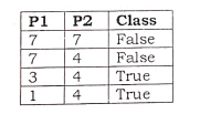
b) Perform the KNN Classification on following dataset and predict the class of X(P1=3,P2=7). Where k=3.

To predict the class of X (P1=3, P2=7) using KNN with k=3, we follow these steps:

Calculate the Euclidean distance between X and all the data points:

Distance(X, P1) = sqrt((3-7)^2 + (7-7)^2) = 4

Distance(X, P2) = sqrt((3-7)^2 + (7-4)^2) = 4.24

Distance(X, P3) = sqrt((3-3)^2 + (7-4)^2) = 3

Select the k nearest neighbors based on the calculated distances:

Nearest neighbors: P3, P1, P2

Determine the majority class among the nearest neighbors:

Class(P3) = True

Class(P1) = False

Class(P2) = False

The majority class among the nearest neighbors is False. Therefore, the predicted class for X is False.

c) How various classifiers can be combined? Explain.

Various classifiers can be combined using ensemble methods. Ensemble methods aim to improve the overall predictive performance by combining the predictions of multiple individual classifiers. There are different ways to combine classifiers, including:

Voting: Each classifier in the ensemble makes predictions, and the class that receives the majority of votes is selected as the final prediction. This can be done through majority voting, weighted voting, or soft voting, depending on the nature of the problem.

Bagging (Bootstrap Aggregating): Multiple classifiers are trained on different subsets of the training data using bootstrapping (sampling with replacement). The final prediction is obtained by averaging or voting on the predictions of each classifier.

Boosting: Classifiers are trained sequentially, where each subsequent classifier is focused on correcting the mistakes made by the previous classifiers. The final prediction is obtained by combining the weighted predictions of all the classifiers.

Stacking: In stacking, multiple classifiers are trained, and their predictions serve as inputs to a meta-classifier, which combines the predictions to make the final decision.

Ensemble methods can lead to improved accuracy, robustness, and generalization of the model by leveraging the strengths of different classifiers and reducing the impact of individual classifier weaknesses.

Q4 a) Explain Decision Tree Algorithm with an example.

The Decision Tree algorithm is a popular supervised learning algorithm used for classification and regression tasks. It builds a tree-like model of decisions and their possible consequences based on the input features.

Example: Let's consider a dataset of car properties (color, type, origin) and whether the car was stolen or not.

1. Begin with the entire dataset as the root node.
2. Select a feature that best splits the dataset based on certain criteria (e.g., information gain, Gini impurity).
3. Create a branch for each possible value of the selected feature.
4. Recursively repeat steps 2 and 3 for each subset of data in the branches until a stopping criterion is met (e.g., reaching a maximum depth, minimum number of samples).
5. Assign the majority class of the training samples in each leaf node as the predicted class.

The decision tree builds a tree structure where each internal node represents a decision based on a specific feature, and each leaf node represents a class label. The tree can be visualized, and it provides interpretable rules for classification.

b) What is Bayes Theorem? How it is useful machine learning?

Bayes Theorem is a fundamental concept in probability theory that calculates the conditional probability of an event given prior knowledge or evidence. In machine learning, Bayes Theorem is used in various algorithms, especially in Bayesian methods and probabilistic models.

The formula for Bayes Theorem is:

P(A|B) = (P(B|A) * P(A)) / P(B)

• P(A|B) represents the posterior probability of event A given event B.
• P(B|A) is the likelihood, which is the probability of observing event B given event A.
• P(A) is the prior probability of event A.
• P(B) is the probability of observing event B.

Bayes Theorem is useful in machine learning as it provides a way to update prior beliefs or probabilities based on new evidence or observations. It is widely used in Bayesian inference, Naive Bayes classifiers, and other probabilistic models.

c) For the given dataset apply the Naive Bayes Algorithm and predict the outcome for a car (Red, Domestic, SUV).

(Answering in later in this video)

Q5 a) Differentiate between classification and clustering process. 

Classification and clustering are two different processes used in machine learning and data analysis:

Classification:

• Classification is a supervised learning task where the goal is to assign predefined labels or categories to input data based on their features.
• The process involves training a model on labeled training data to learn the patterns and relationships between the features and the labels.
• The trained model can then be used to predict the labels of unseen data.

Clustering:

• Clustering is an unsupervised learning task where the goal is to group similar data points together based on their intrinsic characteristics.
• The process involves finding the underlying structure or patterns in the data without any predefined labels.
• Clustering algorithms group data points based on their similarity or distance metrics, aiming to maximize the similarity within clusters and minimize the similarity between clusters.

b) Discuss K-means clustering with example.  

K-means clustering is a popular clustering algorithm that aims to partition a given dataset into K clusters, where K is predefined by the user:

Example:

Let's say we have a dataset of customer information, including age and income. We want to group similar customers based on these attributes.

1. Choose the value of K, which represents the number of clusters we want to create.
2. Randomly initialize K cluster centroids.
3. Assign each data point to the nearest centroid based on their distance.
4. Recalculate the centroids by taking the mean of all data points assigned to each cluster.
5. Repeat steps 3 and 4 until convergence or a maximum number of iterations.

The algorithm iteratively updates the cluster assignments and centroid positions to minimize the within-cluster sum of squares. Eventually, the data points will be grouped into K clusters, where each cluster represents a distinct segment of customers based on age and income.

c) What is the difference between generative and discriminative model? 

The difference between generative and discriminative models lies in their underlying principles and objectives:

Generative Model:

• Generative models learn the joint probability distribution of the input features and the corresponding labels.
• They aim to model the underlying process that generates the data and can generate new samples.
• Given the input features, a generative model can estimate the likelihood of different labels.
• Examples of generative models include Naive Bayes, Hidden Markov Models, and Gaussian Mixture Models.

Discriminative Model:

• Discriminative models directly learn the decision boundary between different classes or labels.
• They focus on learning the conditional probability distribution of the labels given the input features.
• Discriminative models aim to find the most optimal decision boundary that separates different classes.
• Examples of discriminative models include Logistic Regression, Support Vector Machines, and Neural Networks.

Q6 Write short notes on the following: 

a) Dimension Reduction in Machine learning

Dimension reduction is a technique used in machine learning to reduce the number of input features or variables while preserving the relevant information. It helps in simplifying the complexity of the data and improving the efficiency and effectiveness of machine learning models. There are two main approaches to dimension reduction: feature selection and feature extraction.

1. Feature Selection: This approach involves selecting a subset of the original features based on their relevance to the target variable. The selected features are retained, while the irrelevant or redundant ones are discarded. This helps in reducing the dimensionality of the data and eliminating noise or irrelevant information.
   
   
2. Feature Extraction: This approach aims to transform the original high-dimensional data into a lower-dimensional space by creating new features that capture the most important information. Techniques such as Principal Component Analysis (PCA) and Singular Value Decomposition (SVD) are commonly used for feature extraction.

Dimension reduction offers several benefits, including faster computation, improved model performance, better visualization of data, and alleviation of the curse of dimensionality. However, it is important to carefully select the appropriate dimension reduction technique based on the characteristics of the data and the requirements of the problem.

b) Classification Errors

Classification errors refer to the mistakes made by a machine learning model when predicting the class or category of a given sample. In classification tasks, the model aims to assign a class label to each input based on its features. Classification errors can occur in two ways:

False Positive: This error occurs when the model predicts a positive class for a sample that actually belongs to the negative class. It is also known as a Type I error or a "false alarm."

False Negative: This error occurs when the model predicts a negative class for a sample that actually belongs to the positive class. It is also known as a Type II error or a "miss."

The choice of the error metric depends on the specific problem and the consequences of different types of errors. Commonly used error metrics include accuracy, precision, recall, F1 score, and area under the ROC curve. The evaluation of classification errors helps in assessing the performance and reliability of the model and guides improvements in the learning process.

c) Principal Component Analysis (PCA)

Principal Component Analysis (PCA) is a dimensionality reduction technique used to transform a high-dimensional dataset into a lower-dimensional space while retaining as much of the original variance as possible. It aims to find a set of orthogonal axes, known as principal components, along which the data varies the most.

The steps involved in PCA are as follows:

Standardize the data: Normalize the features to have zero mean and unit variance.

Compute the covariance matrix: Calculate the covariance between each pair of features.

Compute the eigenvectors and eigenvalues: Find the eigenvectors and eigenvalues of the covariance matrix. The eigenvectors represent the principal components, and the corresponding eigenvalues indicate the amount of variance explained by each component.

Select the desired number of principal components: Determine the number of principal components to retain based on the desired level of dimensionality reduction.

Transform the data: Project the data onto the selected principal components to obtain the lower-dimensional representation.

PCA has several applications, including data visualization, noise reduction, feature extraction, and data compression. It is widely used in various domains, such as image processing, signal processing, and pattern recognition, to simplify complex data and reveal underlying patterns or structures.

Q7 a) Write short note on Reinforcement Learning using diagram 

Reinforcement Learning (RL) is a type of machine learning where an agent learns to make decisions through trial and error in an environment. The agent interacts with the environment by taking actions and receiving feedback in the form of rewards or penalties. The goal of RL is to find an optimal policy that maximizes the cumulative reward over time.

In RL, the agent learns through a process called the RL loop, which consists of the following steps:

1. Observation: The agent observes the current state of the environment.
2. Action: Based on the observed state, the agent selects an action to perform.
3. Feedback: The agent receives feedback from the environment in the form of a reward or penalty.
4. Update: The agent updates its knowledge or policy based on the received feedback.
5. Repeat: The agent continues the loop by observing, taking actions, and updating until it learns the optimal policy.

The RL process can be visualized using a diagram called the RL loop diagram. It represents the flow of information and actions between the agent and the environment, showcasing the cyclic nature of the learning process.

b) How ADA boosting helps in improvement in classification process? Explain.

AdaBoost (Adaptive Boosting) is a boosting algorithm used in machine learning for improving the classification process. It works by combining multiple weak classifiers to create a strong classifier. The main idea behind AdaBoost is to give more weight to misclassified instances and focus on the difficult examples during subsequent iterations.

The steps involved in AdaBoost are as follows:

1. Assign initial weights: Each instance in the training set is assigned an equal weight.
2. Train weak classifiers: A series of weak classifiers are trained on the data.
3. Evaluate weak classifiers: The performance of each weak classifier is evaluated on the training set.
4. Update instance weights: Instances that are misclassified are assigned higher weights, while correctly classified instances are assigned lower weights.
5. Combine weak classifiers: The weak classifiers are combined into a strong classifier based on their individual performance and instance weights.
6. Repeat: Steps 3-5 are repeated for a specified number of iterations or until a desired level of accuracy is achieved.

AdaBoost helps in improving the classification process by focusing on the challenging instances and giving them more importance during training. By iteratively adjusting the instance weights and combining weak classifiers, AdaBoost can effectively handle complex classification tasks and achieve higher accuracy compared to using a single classifier.

c) Differentiate between PCA and ICA using suitable example.

PCA (Principal Component Analysis) and ICA (Independent Component Analysis) are both dimensionality reduction techniques used in machine learning, but they have different underlying principles and applications.

PCA:

• PCA is a linear transformation technique that aims to find a new set of orthogonal axes (principal components) that captures the maximum variance in the data.
  
  
• It projects the data onto these components, where the first component explains the most variance, the second component explains the second most variance, and so on.
  
  
• PCA is commonly used for feature extraction, data compression, and data visualization.
  
  
• It does not assume any specific distribution of the data.

ICA:

• ICA is a statistical technique that aims to separate a set of mixed signals into their underlying independent components.
  
  
• It assumes that the observed data is a linear combination of independent source signals, and it seeks to estimate the original sources.
  
  
• ICA is useful for tasks such as blind source separation, speech recognition, and image denoising.
  
  
• It relies on the statistical independence assumption and assumes that the sources have a non-Gaussian distribution.

To illustrate the difference between PCA and ICA, consider an example of cocktail party problem. Assume you have a recording of multiple people speaking simultaneously. PCA would aim to find the principal components that capture the maximum variance in the mixture of voices, while ICA would attempt to separate the individual voices by estimating the independent source signals.

Q8 a) Differentiate between value iteration and policy iteration.

Value iteration and policy iteration are two common algorithms used in reinforcement learning for solving Markov decision processes (MDPs) and finding optimal policies.

Value iteration:

• Value iteration is an iterative algorithm that calculates the optimal value function by repeatedly updating the values of states.
• It starts with an initial estimate of the value function and iteratively improves it until convergence.
• In each iteration, the algorithm updates the value of each state by considering all possible actions and their corresponding expected returns.
• Value iteration converges to the optimal value function and policy.

Policy iteration:

• Policy iteration is an iterative algorithm that alternates between policy evaluation and policy improvement steps.
• It starts with an initial policy and iteratively improves it by evaluating and updating the value function.
• In the policy evaluation step, the algorithm calculates the value function for the current policy.
• In the policy improvement step, the algorithm updates the policy by selecting the action that maximizes the expected return.
• Policy iteration converges to the optimal policy and value function.

The main difference between value iteration and policy iteration is in their update process. Value iteration directly updates the value function in each iteration, while policy iteration updates the policy based on the current value function.

b) What are policy search?

Policy search refers to a class of reinforcement learning methods that learn policies directly, without explicitly estimating the value function. Instead of estimating the value function, policy search methods directly optimize the policy parameters to find the best policy for the given task.

Policy search algorithms explore the policy parameter space to search for the policy that maximizes the expected return. They use different optimization techniques, such as gradient ascent or evolutionary algorithms, to update the policy parameters based on the observed rewards.

Policy search methods have the advantage of being able to handle high-dimensional or continuous action spaces, and they can learn complex policies. They are commonly used in applications where the reward function is not easily defined or the environment dynamics are uncertain.

c) Explain LQR and LQG Model of Learning.

LQR (Linear Quadratic Regulator) and LQG (Linear Quadratic Gaussian) are models of learning that are used in control theory.

LQR:

• LQR is a control strategy for continuous-time linear systems with quadratic cost functions.
• It aims to find an optimal control policy that minimizes a quadratic cost function, considering the system dynamics and control constraints.
• LQR uses the dynamic programming principle and the Riccati equation to compute the optimal control gains.

LQG:

• LQG is an extension of the LQR framework that incorporates uncertainty in the system dynamics and sensor measurements.
• It considers a linear system with Gaussian noise in the dynamics and measurements.
• LQG combines the LQR control policy with a Kalman filter that estimates the system state based on noisy measurements.
• The LQG controller adjusts the control action based on the estimated state to optimize the system performance.

LQR and LQG models are widely used in control systems engineering and provide robust and optimal control solutions for linear systems with noise and uncertainties.

                                      -------------------